Introduction to System Dynamics

• Simulations in biology, ecology or economy:
  • highly complex systems
  • causal relationships often unclear
  • simulation as testbed to check new ideas
  • mathematical formulation
    • usually as differential equation
    • often too abstract for users
    • functional relationships often based on empiric data (tables, plots)
  • graphical modeling with system dynamics diagramms
    • emphasis on causal relationships
    • only very few general blocks
    • mathematical relations are hidden, equations are defined as parameters
    • several commercial modeling and simulation environments, e. g. Stella, Vensim, Simile
  • invented by Jay Forrester around 1955
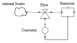
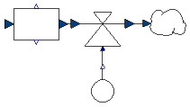
• Basic building blocks of system dynamics diagrams:
  • Reservoir (or stock)
    • corresponds to a state variable
    • needs initial value
  • Flow
    • defines rate of change (positive/negative) of a reservoir
    • connects reservoir with another reservoir or external sources/sinks (cloud)
    • is symbolized as a valve
  • Converter
    • external parameter or auxiliary variable
    • computed using other values
    • concrete computation is hidden as parameter
  • Connector
    • specifies, which variables affect others
  • graphical representation
    • 
• Physical modeling:
  • models built from "physical" components (masses, resistors, valves) instead of integrators or function blocks
  • connecting lines represent "physical" connections (flanges, wires, pipes) instead of signals
  • internal representation uses Modelica language
    • object-oriented, equation-based modeling language
    • provides means for graphical representation of components and models
    • huge free library of components (MSL = Modelica standard library)
  • simulation
    • equations come from components and connections
    • automatically combined, simplified (highly non-trivial!) and numerically solved
  • modeling and simulation environment
    • several commercial programs
    • open source: OpenModelica
• Modelica library SystemDynamics.mo:
  • based on SystemDynamics 2.0 by Cellier
  • design changed to cope with blocks like Oven
  • using library in OpenModelica
    • start OMEdit
    • load base library SystemDynamics.mo und examples library SystemDynamicsExamples.mo
    • both are displayed in Libraries pane
  • design of base library
    • packages Reservoirs, Flows and Converters
    • predefined components for common equations
    • user-defined components necessary for special mathematical relations
    • definition of such components easy
    • packages Interfaces contains supporting auxiliary components
  • design of example library
    • Examples contains executable models
    • packages Examples for executable models,  AuxComponents for auxiliary components
    • required data sets in package Resources
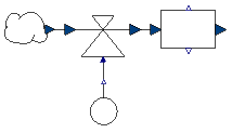
• Simple growth model Inflow:
  • only one state variable
  • growth (inflow)
    • defined by flow (valve symbol)
    • rate variable (i. e. amount/time)
  • defined by ConstantConverter
  • diagram
    • 
• Building the model:
  • pick up components from library pane and drag them into model pane
    • form Reservoirs: Stock, CloudSource
    • from Flows: Flow
    • from Converters: ConstantConverter
  • connect components
  • set parameter values (after double click on a component)
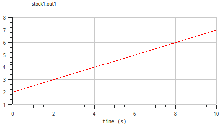
    • initial value of reservoir (Stock): m0 = 2
    • inflow rate (ConstantConverter): constValue = 0.5
• Running simulation:
  • check model
  • setup and run simulation
    • Stop Time = 10
    • automatically runs simulation
    • → one output window is shown
  • change window size (plot window icons "hidden" top-right)
  • choose variable: Inflow.stock1.out1
    • 
  • use switch at bottom-right to retrun to model pane
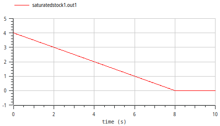
• Model Outflow:
  • mirror image of Inflow
    • 
    • initial value m0 = 4
  • simulation
    • stock value becomes negative
    • is a negative level meaningful?
  • alternative: use SaturatedStock with  minLevel = 0
  • result
    •