Predator prey systems

• Modeling of predator and prey populations:
  • state variables N_b, N_r for number of prey and predator animals
  • inflows for births, outflows for deaths
  • flows like in population models
    • constant birth and death rates
    • number of births and deaths proportional to size of population
  • interaction between the two species
    • F = number of prey hits
    • proportional to  N_b and N_r
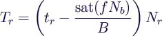
    • directly increases number of prey deaths T_b
    • decreases number of predator deaths T_r
    • demand B = number of prey animals (per time) needed by a predator to survive
  • concrete relations (Lotka-Volterra equations)
    • 
  • model PredatorPrey1
    • 
  • results
    • 
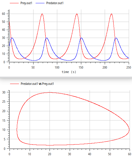
    • typical oscillations
    • closed loop in phase diagram ≙ constant of motion
  • increase of initial number of prey animals from 50 to 500
  • • 
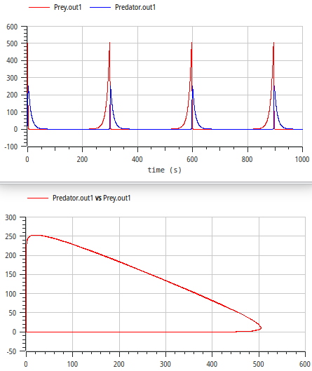
    • reduce solver tolerance to 1e-8 !
    • N_r rises immediately
    • both populations collapse but recover after a long time
    • very steep oscillations
    • still a closed loop in phase diagram
    • very unnatural behaviour!
  • problem
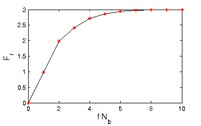
    • number of catches per predator F_r = F / N_r = f N_b rises with N_b
    • idea: limit F_r to a saturation value F_r,max
• Functions defined by graphs:
  • saturation curve F_r = sat(f N_b) known only qualitatively
  • defined explicitely by a set of  points and linear interpolation
    • 
  • implemented with component Mult2GraphConverter
    • multiplies its inputs and applies interpolated function to the product
    • points defined in catchesPerPredator.txt
    • values defined in Modelica as constant array in SystemDynamicsExamples.Resources.PredatorPrey.cpp
• Results of PredatorPrey2B:
  • N_b(0) = 50 → same results as before (F_r far from saturation)
  • N_b(0) = 500
    • 
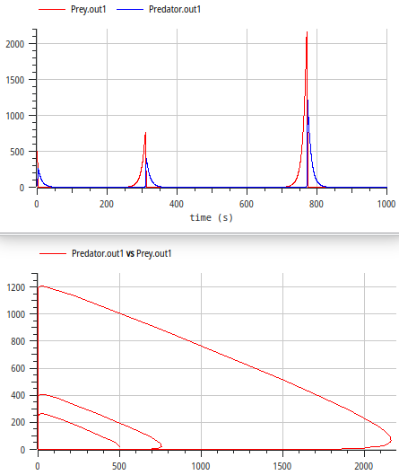
    • oscillations get stronger!
  • reason: T_r becomes negative
    • 
  • happened already for PredatorPrey1, but caused limited damage due to constant of motion