Coupling of conveyors with different velocities

• Problem:
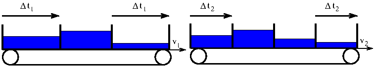
  • two coupled conveyors, lengths l_1,2 and constant velocities v_1,2
  • continuous process for connected conveyors
    • 
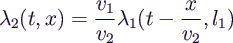
    • → simply change line load λ₂ by factor v₁/v₂
  • discrete process with different l_E1,2 and ∆t_1,2
    • conveyor 1 sends entities with time intervals ∆t₁
    • conveyor 2 outputs entities with time intervals ∆t₂
  • timing doesn't fit
    • 
• Basic idea:
  • entity ≙ content of a given compartment on a conveyor
    • created and filled at the entrance
    • emptied and destroyed at the exit
  • how to compute mass m_out of a new entity for conveyor 2?
  • requirements
    • mass conservation on short time scale
    • homogeneity, i. e. output distribution similar to input
  • crucial parameter
    • 
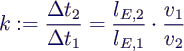
    • k > 1 → add up incoming masses to one compartment
    • k < 1 → distribute incoming mass to several compartments
  • simple case k∊ℕ → add up k incoming masses
  • simple case 1/k∊ℕ → distribute incoming mass to 1/k outgoing masses
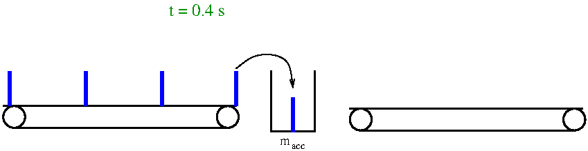
• Strategy for k > 1:
  • introduce virtual bin with mass m_acc between conveyors
  • incoming entities fill bin
  • outgoing entity empties bin
  • example
    • l_E1 = l_E2 = 1 m, v₁ = 2.5 m/s, v₂ = 1 m/s, m_in ≡ 1 kg
    • →  ∆t₁ = 0.4 s, ∆t₂ = 1 s, k = 2.5
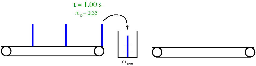
• Strategy A for k < 1:
  • again virtual bin with mass m_acc between conveyors
  • each time m_in arrives: compute partition mass m_p
    
    • m_p = k m_in
  • mass of outgoing entity
    • m_out = min(m_p, m_acc)
  • good example
    • ∆t₁ = 1 s, ∆t₂ = 0.35 s → k = 0.35
    • very homogenous distribution
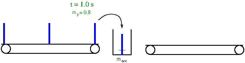
  • bad example
    • ∆t₁ = 1 s, ∆t₂ = 0.8 s → k = 0.8
    • m_acc grows → short time mass conservation violated
• Strategy B for k < 1:
  • like A, but changed partition size
    • m_p = k m_acc
    • distribute the surplus of m_acc
  • precise mathematical description in paper
  • bad example (k = 0.8)
  • comparison
    • 
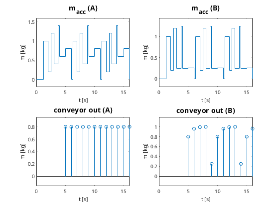
    • B: much better short time mass conservation
    • A: better homogeneity